Illegal Logging Detection Using Vertex AI Audio Model

Ever wondered if we could hear illegal logging in a forest before anyone sees it? In this tutorial, we’ll walk through building an audio classifier that can detect wood-logging sounds (like chainsaws and axes) using Google Cloud’s Vertex AI. We’ll use a real bioacoustics dataset and transform audio into images (spectrograms) to train a model — all without building a neural network from scratch. Let’s dive in!

Use Case and Dataset

Imagine we have solar-powered audio recorders scattered across a protected forest. They continuously capture ambient sounds. Our goal is to automatically spot manual wood logging activity (e.g. the sound of chainsaws or axes) amid all the other forest noises. This could alert rangers to illegal logging in real time. To build this, we need a robust dataset of forest sounds to train our model.

FSC22 is a public benchmark dataset of forest environment audio designed for acoustic monitoring. It contains 2,025 audio clips, each 5 seconds long, covering a wide variety of forest sounds. These clips are organized into 6 main categories (with 34 fine-grained classes) covering everything from animal calls to weather and machinery. Notably for us, one category is Mechanical Sounds (e.g. axe, chainsaw, handsaw, generator) — basically the kinds of tools used in wood logging. Another category (Forest Threats Sounds) even includes wood chopping noises. FSC22 was chosen because it specifically targets forest acoustics and includes the kinds of logging-related sounds we care about. It was created to fill the lack of a dedicated forest audio dataset, with carefully annotated clips for consistent labels.

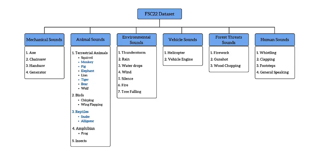
Figure: Taxonomy of the FSC22 forest sound dataset. The dataset covers a broad range of forest sounds organized into 6 groups (mechanical, animal, environmental, vehicle, threat, and human sounds). Notice Mechanical Sounds includes tools like chainsaws, axes, and handsaws — key indicators of logging activity.

For our project, we’ll simplify the task to a binary classification: “Wood Logging” vs “Not Wood Logging”. Using the FSC22 data, we map any audio from chainsaws, axes, handsaws, or related wood-cutting sounds into the Wood-Logging class, and all other sounds (birds chirping, rain, wind, human voices, etc.) into the Non-Logging class. This gives us a focused dataset to train our detector: positive examples of logging noises and plenty of negative examples of normal forest ambiance.

Preprocessing Audio into Mel Spectrograms

Why spectrograms? We’re going to convert each audio clip into a Mel spectrogram image in order to train an image-based model. Raw audio is just a wave, but a spectrogram turns it into a picture of sound: time on the x-axis, frequency on the y-axis, and intensity shown by color. This visual representation makes it easier for a convolutional neural network (CNN) to learn patterns, just like it would on a photo. In fact, researchers found that using Mel spectrogram features with CNNs yielded high accuracy (over 92% in some cases) for classifying forest sounds! The Mel scale is also inspired by human hearing, emphasizing frequencies in a way that makes important sound features stand out.

Step 1: Download and label the audio. We start by downloading the FSC22 clips (the authors have made them freely available). In a Vertex AI Workbench notebook, we fetch the audio files (e.g., from a cloud storage or Kaggle link) using a provided script/notebook.

# Download latest version
path = kagglehub.dataset_download("irmiot22/fsc22-dataset")
print("Path to dataset files:", path)

We then organize the files into two folders or lists: one for wood-logging sounds (chainsaw, axe, etc.) and one for non-logging sounds. Each audio file retains its original class label from FSC22, which we’ll use to decide which group it belongs in. For example, an audio labeled “chainsaw” or “wood chopping” will be mapped to the Wood-Logging category, whereas “bird chirping” or “rain” will be mapped to Non-Logging. This way, we create a clean training set with our two target classes.

Step 2: Convert audio to Mel spectrograms. Now for the fun part — turning each audio clip into an image. We use a Python script (let’s call it create_melspec.py) to do this conversion in bulk. The script uses Librosa, a popular audio processing library. For each WAV file, we load the audio at 16 kHz sampling rate (uniform sample rate for consistency) and then compute a Mel-scaled spectrogram with a set number of frequency bands (here we use 128 mel bands). We then apply a logarithmic dB transform to the spectrogram so that the values represent decibel intensity (this helps compress the huge range of raw audio power into a more manageable scale).

# Load audio at 16 kHz
y, sr = librosa.load(input_path, sr=16000)

# Generate mel spectrogram (128 mel bands) and convert to decibels
mel_spec = librosa.feature.melspectrogram(y=y, sr=sr, n_mels=128)
mel_spec_db = librosa.power_to_db(mel_spec, ref=np.max)

In just a few lines, we go from waveform y to a matrix mel_spec_db that represents the sound’s frequency content over time. To make this into an image, the script then plots the spectrogram matrix as an image (using Matplotlib) and saves it to file – one PNG image per audio clip, stored in a folder corresponding to its class label. The resulting Mel spectrogram image is essentially a heatmap: time runs left to right, frequency (low to high) bottom to top, and the intensity of each frequency at each moment is shown by color brightness. For example, a chainsaw clip might produce a spectrogram with constant high-frequency energy (a bright band across the top), while an axe chopping sound might show distinct mid-frequency bursts corresponding to each chop. Each 5-second audio yields a spectrogram image ~ a few hundred pixels wide (depending on hop length) by 128 pixels tall (for 128 mel bands).

Now we have a directory of spectrogram images for all our audio clips. These images are labeled and sorted into two top-level folders (Wood-Logging vs Non-Logging). The data is ready for the machine learning stage!

Creating a Vertex AI Dataset

With our images prepared, we move to Vertex AI on Google Cloud, which will handle the model training. First, we need to get the data into Vertex AI:

1. Create an “input manifest” (CSV): To bulk import data into Vertex AI, it helps to have an input CSV file listing each image’s GCS path and its label. We generate a CSV where each line has the format:gs://path/to/image.png, label. For instance:

gs://my-audio-logging-project/spectrograms/Wood-Logging/chainsaw_123.png, Wood-Logging  
gs://my-audio-logging-project/spectrograms/Non-Logging/rain_456.png, Non-Logging  
... (and so on for all images) ...

This manifest file will let Vertex AI know where the images are and what their labels are. Creating this file ahead of time makes the import process easy — instead of manually uploading or labeling images one by one in the interface, we can just point Vertex to this file and it will import all our data with the labels attached.

Training an AutoML Model on Vertex AI

Vertex AI offers an AutoML training service that trains a model on our dataset with minimal effort from us. We’ll use this to create our audio classifier model:

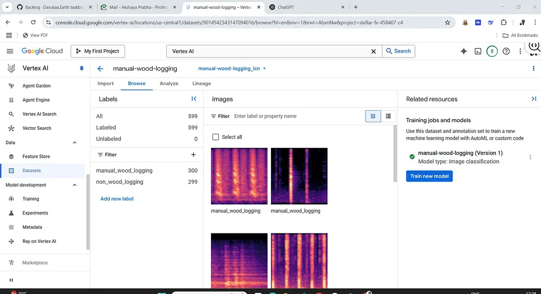
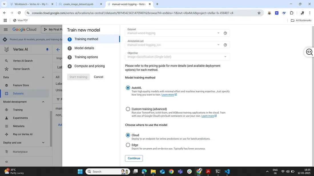
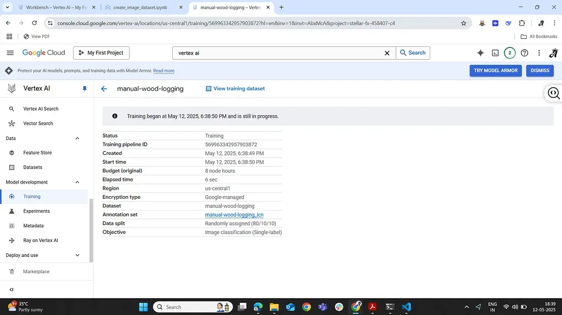
1. Initiate training: In the Vertex AI dataset page, we click Train new model. We choose AutoML image classification (this uses Google’s AutoML Vision under the hood to find the best model). We then go through the steps of the training wizard. Step 1: Select the dataset (our forest spectrogram dataset) and confirm the objective (single-label classification). Step 2: Choose a training method — we’ll stick with AutoML (as opposed to a custom training job) since we want Google to automatically handle model selection and tuning for us.

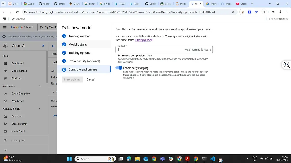
2. Configure training settings: We give our model a name (e.g. “logging-sound-detector”) and choose a compute budget. Vertex AI allows you to set how many node-hours to train for — basically how much time it should spend trying different model architectures. A typical setting might be 8 or 24 node-hours for a small dataset, but you can adjust depending on how much you’re willing to spend. (It will also show the approximate cost for that training run — always good to double-check! Vertex AI is a paid service, and longer training = higher cost). We can also choose to enable early stopping so it doesn’t use the full budget if the model stops improving.

3. Launch training and wait: Once we confirm settings, we start the training job. Now Vertex AI handles everything: it will spin up GPU-powered machines, try out model architectures (likely various CNN models since this is an image task), and train and evaluate them using part of our dataset. For our dataset size, this training might take on the order of tens of minutes to a few hours, depending on the budget.

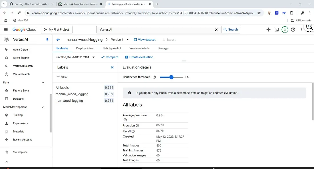
4. Monitor and evaluate: Vertex AI will automatically keep aside a portion of the data for validation. After training completes, Vertex will present the evaluation results — e.g. an overall accuracy, a confusion matrix, and per-class precision/recall. In our case, with a clear-cut distinction between logging tool noises and other sounds, we expect high performance. (If the dataset is good, the model might achieve excellent accuracy distinguishing these two classes, since chainsaw or axe sounds are quite distinct from natural forest sounds.)

5. Deployment (optional): Once satisfied, we can deploy the model to an endpoint for serving predictions. This means we could send new audio clips (converted to spectrograms) to the model and get a prediction of whether it’s Wood-Logging or not. In a real system, you’d automate the conversion of incoming audio streams to spectrogram images and have the model evaluate them. For now, Vertex AI allows you to test the model in the console by uploading an image and seeing the predicted label and confidence.

And that’s it — without writing a single line of model code, we have trained a deep learning model that listens for illegal logging! Vertex AI’s AutoML picked the best CNN for our spectrogram images and optimized it for us. The result is a classifier that can detect the sounds of forest destruction with impressive accuracy. 🎉

(Note: Always keep an eye on your Google Cloud budget; training models on the cloud isn’t free. Vertex AI will show you the cost estimation before you start.)

Pros and Cons of Using Vertex AI

Every tool has its strengths and trade-offs. Here’s a quick summary of Vertex AI AutoML’s pros and cons for this project:

Pros:

Ease of Use: Minimal coding, automated model selection.
Rapid Development: Quick transition from data to deployment.
Scalability: Efficient handling of large datasets.

Cons:

Cost: Paid cloud service can become expensive.
Limited Control: AutoML provides limited transparency on model details.
Data Privacy: Data must reside in Google’s Cloud environment.

Conclusion

By leveraging Vertex AI and the FSC22 forest sound dataset, we’ve built a practical audio logging detector in a few straightforward steps. This approach is accessible to ML beginners and bioacoustics enthusiasts alike — combining domain-specific data with cloud AutoML tools. With this classifier, a forest guardian system could automatically hear and flag suspicious logging activity, hopefully helping protect forests through early detection. Happy building, and may your models always listen well!

Reference:

Bandara, Meelan, Roshinie Jayasundara, Isuru Ariyarathne, Dulani Meedeniya, and Charith Perera. “Forest sound classification dataset: Fsc22.” Sensors 23, no. 4 (2023): 2032. https://www.mdpi.com/1424-8220/23/4/2032

Detecting Illegal Logging Sounds with an Audio Classifier on Vertex AI