Beyond Pixels: A New Era of Geospatial Reasoning with AlphaEarth’s Embedding Calculus

For decades, the fundamental unit of satellite remote sensing has been the pixel. We’ve mastered the art of classifying them, tracking their changes, and assembling them into static maps. But this approach has always had a limitation: it’s like trying to understand a movie by looking at individual frames. We see the state of the world, but we struggle to capture the fluid, continuous process of its transformation.

Today, that paradigm is changing. The release of the AlphaEarth Foundations model and its embedding datasets in Google Earth Engine provides us with a new language to describe our planet — a language where we can move from static description to dynamic reasoning.

This article is a technical deep dive into a new methodology we’re calling “Geospatial Calculus.” We’ll demonstrate how to go beyond pixels and mathematically model the very process of deforestation as a single vector. I’ll walk you through the entire workflow, from the underlying theory to the executable Earth Engine code, and show how this technique unlocks a continuous, global measure of forest health and a predictive tool for finding deforestation hotspots.

The Foundation: Why AlphaEarth Embeddings are a Paradigm Shift

To understand the “how”, we must first grasp the “why.” The GOOGLE/SATELLITE_EMBEDDING/V1/ANNUAL ImageCollection is not just another set of bands. It’s the output of a foundational model that has learned a deep, multi-modal representation of the Earth’s surface.

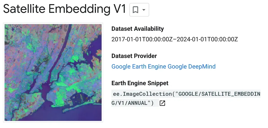
Satellite Embedding dataset in the Earth Engine Data Catalog.

As detailed in the AlphaEarth Foundations paper, the model ingests a full year of time-series data from a suite of sensors (Sentinel-1, Sentinel-2, Landsat, ERA5 climate data, and more) for every 10m pixel. It then compresses this immense spatiotemporal information into a 64-dimensional vector, or embedding.

Think of this 64-number signature as the “geospatial DNA” of a location. It encodes not just spectral color, but also its texture, structure, moisture content, and, crucially, its annual rhythm or phenology. The model has created a rich, semantic space where the distance and direction between these embedding vectors have profound, real-world meaning. This is the property we will exploit.

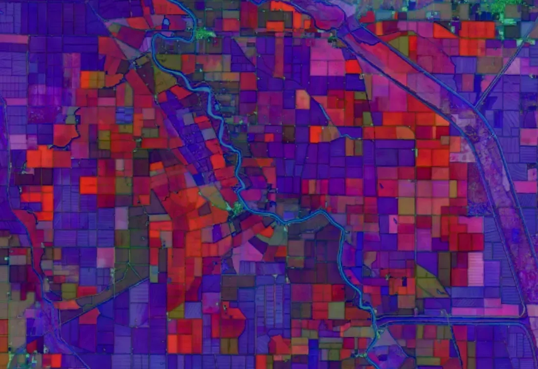
Examples for Agricultural land in Central California, USA, embedding layer for the years 2024 (Source: Earth Engine Code Editor script)

The Methodology: From Feature Vectors to Vector Arithmetic

Our experiment rests on a powerful hypothesis: if we can identify the average embedding for a “pristine” state and an “altered” state, the vector connecting them mathematically represents the process of alteration.

Step 1: Defining Our Anchors with Scientific Rigor

We need an objective, repeatable way to define our two states: Pristine Forest and Recently Deforested. The Hansen et al. Global Forest Change dataset provides the perfect, peer-reviewed source for this. We define our anchors within the Amazon, a region with a strong, clear signal for both states.

import ee
import geemap
import numpy as np

# Initialize Earth Engine
geemap.ee_initialize()

# Load the Hansen GFC dataset, our source of ground truth
gfc = ee.Image('UMD/hansen/global_forest_change_2022_v1_10')

# Define 'Pristine Forest': High canopy cover (>80%) in 2000 and zero loss.
pristine_forest_mask = gfc.select('treecover2000').gt(80).And(gfc.select('loss').eq(0))

# Define 'Recently Deforested': Was dense forest, but lost in the last 5 years.
# 'lossyear' is encoded as years since 2000 (e.g., 18 = 2018)
recent_loss_mask = gfc.select('treecover2000').gt(80).And(gfc.select('lossyear').gte(18))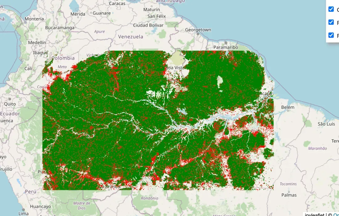

Anchor masks for Pristine Forest (green) and Recently Deforested land (red) derived from the Hansen GFC dataset over the Amazon Basin. These regions serve as our ground truth for calculating the process vector.

Step 2: Calculating the Mean Embeddings

Next, we load the 2023 AlphaEarth embeddings and calculate the average embedding vector for all pixels within our two masks. By averaging over millions of pixels, we capture the stable, quintessential signature of each state, filtering out local noise.

# Load the 2023 AlphaEarth Embedding Image
YEAR = 2023
embeddings_image = ee.ImageCollection('GOOGLE/SATELLITE_EMBEDDING/V1/ANNUAL') \
    .filter(ee.Filter.date(f'{YEAR}-01-01', f'{YEAR}-12-31')).mosaic()
band_names = embeddings_image.bandNames()

# Define a large region for a stable calculation
amazon_roi = ee.Geometry.Polygon(
    [[[-75, -10], [-75, 5], [-50, 5], [-50, -10]]], None, False)

# Use reduceRegion to get the mean vector for each class
mean_pristine_dict = embeddings_image.updateMask(pristine_forest_mask).reduceRegion(
    reducer=ee.Reducer.mean(), geometry=amazon_roi, scale=1000, maxPixels=1e9)

mean_deforested_dict = embeddings_image.updateMask(recent_loss_mask).reduceRegion(
    reducer=ee.Reducer.mean(), geometry=amazon_roi, scale=1000, maxPixels=1e9)

# Pull results from the server and convert to NumPy arrays for local calculus
mean_pristine_vector = np.array(mean_pristine_dict.values(band_names).getInfo())
mean_deforested_vector = np.array(mean_deforested_dict.values(band_names).getInfo())

# The core calculation: subtracting the start state from the end state
deforestation_vector = mean_deforested_vector - mean_pristine_vector

This deforestation_vector is the cornerstone of our analysis. It is a 64-dimensional vector that encapsulates the average mathematical shift in the embedding space when a forest is cleared.

The Critical Question: How Can a Single Year Capture a Process?

This is a crucial point. We are using data from only one year (2023). How can it capture a process that unfolds over time?

The answer: we use the spatial distribution of the landscape as a proxy for the temporal process. The 2023 landscape is a complete snapshot containing pixels in every state of transition. It has the “before” (pristine forests) and the “after” (cleared lands) coexisting in space. Our vector connects these coexisting states, thereby defining the path of change without needing a multi-year time-series for a single pixel.

Application 1: A Continuous Global Forest Degradation Index

With our process vector defined, we can now use it as a probe. By calculating the cosine similarity (a dot product) of every forest pixel’s embedding with our deforestation_vector, we are mathematically projecting it onto the path of change. We are asking: “Based on your current DNA, how far along the road to deforestation are you?”

# Normalize the vector to represent a pure direction of change
deforestation_vector_normalized = deforestation_vector / np.linalg.norm(deforestation_vector)
deforestation_ee_image = ee.Image.constant(deforestation_vector_normalized.tolist()).rename(band_names)

# Calculate the dot product across the entire globe
degradation_index = embeddings_image.multiply(deforestation_ee_image).reduce('sum')

# Mask to show only forested areas globally
forest_mask_global = gfc.select('treecover2000').gt(30)
degradation_index_masked = degradation_index.updateMask(forest_mask_global)

The resulting map is not a classification; it is a measurement. It provides a continuous, nuanced view of forest health, revealing subtle degradation that binary maps completely miss.

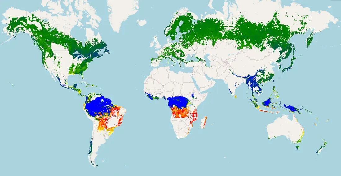
The Global Forest Degradation Index. Red/orange areas indicate forests whose embedding signature is highly aligned with the deforestation vector, signaling high degradation. Blue/green areas represent healthy, intact forests.

Application 2: Predictive Hotspot Detection

Going a step further, we can use the signature of our “cleared land” anchor (mean_deforested_vector) as a target for a global similarity search. This allows us to find all pixels on Earth that, right now, strongly match the signature of a recently cleared patch of the Amazon.

# Create an image representing the target "cleared land" signature
cleared_land_signature = ee.Image.constant(mean_deforested_vector.tolist()).rename(band_names)

# Calculate similarity of every pixel on Earth to this signature
similarity_to_cleared = embeddings_image.multiply(cleared_land_signature).reduce('sum')

# Threshold to find the strongest matches
hotspot_threshold = 0.8
deforestation_hotspots = similarity_to_cleared.gt(hotspot_threshold).selfMask()

This turns our model into a proactive monitoring tool, capable of flagging large-scale land conversion events in near-real-time, providing actionable intelligence for conservation efforts.

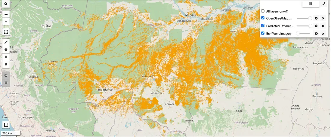
Predicted deforestation hotspots in the Amazon. Orange areas are pixels with a >0.8 cosine similarity to the “cleared land” anchor, indicating active or very recent large-scale land conversion.

Conclusion: The Dawn of Geospatial Calculus

The AlphaEarth embedding dataset does more than just simplify existing workflows; it enables entirely new ones. By treating the Earth’s surface as a learned semantic space, we can move from mapping static states to modeling dynamic processes.

The techniques demonstrated here — defining process vectors through anchor states and using them for projection and similarity search — are a universal toolkit. One can imagine calculating vectors for urbanization, agricultural intensification, glacial retreat, or post-fire recovery.